8. Basic Examples
Here we can find some basic examples of using the methods included in the package.
Note
We suggest using the .shape attribute when running these examples in order to understand the expected
inputs and outputs.
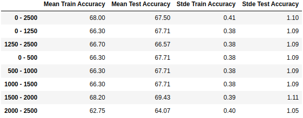
8.1. RMSF Baseline Models
The example below shows how we can evaluate the residue selection using simple and intuitive models implemented on this package. This example should not be used as a model for classifying ligands, only for evaluating residue selections.
Briefly the flow below is:
Read the data
Bootstrap the ligands to create a number of training - validation samples
For each window and bootstrap samples fit and predict on the training and validation set
Create a DataFrame summarizing the results
from MDSimsEval.rmsf_baseline_models import bootstrap_dataset, ResidueMajority, \
    AggregatedResidues
from MDSimsEval.utils import create_analysis_actor_dict

from tqdm import tqdm
from scipy import stats
import numpy as np
import pandas as pd
import pickle

# Read the data
analysis_actors_dict = create_analysis_actor_dict('path_to_data_directory/')


def calculate_accuracy(model, ligands_dict):
    # We define a function that will help us calculate the accuracy of our feature selection
    acc = 0
    for which_agon in ligands_dict['Agonists']:
        label = model.predict(which_agon)
        if label == 1:
            acc += 1

    for which_antagon in ligands_dict['Antagonists']:
        label = model.predict(which_antagon)
        if label == 0:
            acc += 1

    return acc / (len(ligands_dict['Agonists']) + len(ligands_dict['Antagonists'])) * 100


# IMPORTANT: For any RMSF analysis always initialize rmsf_cache as an empty dict and pass it as an argument to the
# rmsf methods
rmsf_cache = {}

# Windows we will evaluate our feature selection on
windows = [[0, 2500], [0, 1250], [1250, 2500], [0, 500], [500, 1000], [1000, 1500], [1500, 2000], [2000, 2500]]

# Create the bootstrap samples
train_dicts, validation_dicts = bootstrap_dataset(analysis_actors_dict, samples=3, sample_size=20)

total_metrics = {}  # We will save our accuracies of each window on this dict

for start, stop in windows:
    accs = []
    model = AggregatedResidues(start, stop, rmsf_cache, method=np.mean)
    # model = ResidueMajority(start, stop, rmsf_cache, np.mean)

    # The loop is slow at each 1st iteration but speeds due to rmsf_cache
    for train_dict, validation_dict in tqdm(list(zip(train_dicts, validation_dicts)), desc=f'Window {start} - {stop}'):
        model.fit(train_dict, residues=np.arange(290))

        accs.append([calculate_accuracy(model, train_dict), calculate_accuracy(model, validation_dict)])

    accs = np.array(accs)  # Transform to numpy array for the mean, sem below
    mean_accs = np.mean(accs, axis=0)

    # Calculating the Standard Error of the Mean gives us an indication of the fluctuations of the accuracies
    # High sem suggests that we need to increase the number of bootstrapped samples
    sem_accs = stats.sem(accs, axis=0)

    # Save the results on the dictionary that will be transformed to a DataFrame
    total_metrics[f'{start} - {stop}'] = [mean_accs[0], mean_accs[1], sem_accs[0], sem_accs[1]]

# Save the results using pickle for future use
with open('cache/baseline_models/aggregated_acc_all_res_mean.pkl', 'wb') as handle:
    pickle.dump(total_metrics, handle)

print(pd.DataFrame.from_dict(total_metrics, orient='index',
                             columns=['Mean Train Accuracy', 'Mean Test Accuracy',
                                      'Stde Train Accuracy', 'Stde Test Accuracy']).round(decimals=2))
Output (if ran on Jupyter Notebook, using display instead of print at the end):
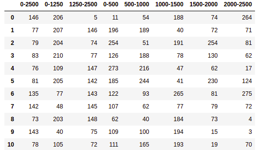
8.2. RMSF Display the top-50KS Residues
In this example the goal is to display the top-10KS residues in descending order of discriminating
importance of their RMSF based on the K-S statistical test performed in the
bootstrapped_residue_analysis method.
from MDSimsEval.rmsf_bootstrapped_analysis import bootstrapped_residue_analysis, find_top
from MDSimsEval.utils import create_analysis_actor_dict

from scipy import stats
import pandas as pd

# Parameters to be set
outer_samples_numb = 500
sample_size = 20  # e.g. if set to 20 each sample contains 20 unique agonists and 20 unique antagonists
top_residues_numb = 10

analysis_actors_dict = create_analysis_actor_dict('path_to_data_directory/')

# IMPORTANT: For any RMSF analysis always initialize rmsf_cache as an empty dict and pass it as an argument to the
# rmsf methods
rmsf_cache = {}

windows = [[1, 2500], [1, 1250], [1251, 2500], [1, 500], [501, 1000], [1001, 1500], [1501, 2000], [2001, 2500]]

important_residues = {}
for start, stop in windows:
    res = bootstrapped_residue_analysis(analysis_actors_dict, start, stop, stats.ks_2samp, threshold=0.05,
                                        samples_numb=outer_samples_numb,
                                        sample_size=sample_size, rmsf_cache=rmsf_cache)
    try:
        # The lines below aggregate the results in order to end up with a sorted list of the most important
        # residues
        flat_res = [residue for iteration_residues in res for residue in iteration_residues]
        res_freqs, __ = find_top(flat_res, top_residues_numb)
        important_residues[f'{start}-{stop}'] = [res_freq[0] for res_freq in res_freqs]
    except IndexError:
        print(f'Not enough significant residues found - Window {start}-{stop}')
        continue

# Pandas transforms the dictionary to an interpretable tabular form
residues_df = pd.DataFrame(important_residues)
print(residues_df)
Output (if ran on Jupyter Notebook, using display instead of print at the end):
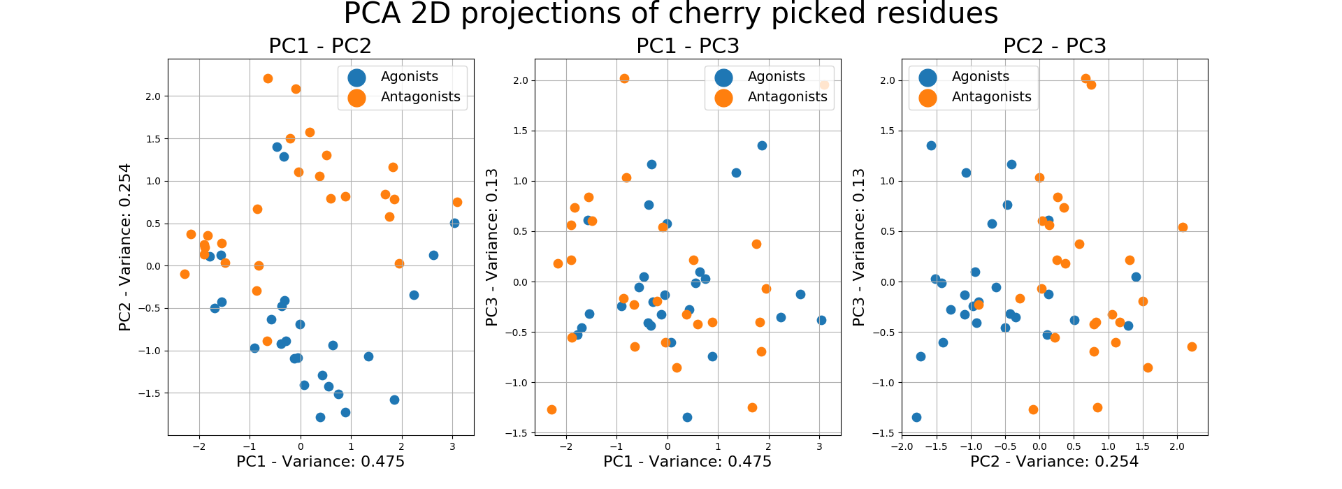
8.3. RMSF Cherry Picked Residues
We define cherry picking as empirically deciding which residues and on which windows we are going to calculate the RMSF of the ligands. The selection of the residues may come from a combination of plots or from the experience in the field.
The example below inputs a dictionary of specific residues on specific windows and creates their 2D PCA projection of their 1st 3 PCs, in order to evaluate their separability.
from MDSimsEval.utils import create_analysis_actor_dict
from MDSimsEval.rmsf_bootstrapped_analysis import find_rmsf_of_residues

from sklearn.decomposition import PCA

import matplotlib.pyplot as plt
import numpy as np


# Reading the agonists and the antagonists
analysis_actors_dict = create_analysis_actor_dict('path_to_data_directory/')

# IMPORTANT: For any RMSF analysis always initialize rmsf_cache as an empty dict and pass it as an argument to the
# rmsf methods
rmsf_cache = {}

# A dictionary of selected residues (keys) and a list of windows (values) that we will use
residues = {
                 115: [[0, 500], [2000, 2500]],
                 117: [[2000, 2500]],
                 81: [[2000, 2500]],
                 78: [[1000, 1500], [1500, 2000]],
                 254: [[0, 500], [1500, 2000]],
            }

# Create an array of the RMSFs of the selected residues on the selected windows
rmsf_array = []
for res, windows in residues.items():
    for window in windows:
        rmsf_array.append(find_rmsf_of_residues(analysis_actors_dict, [res], window[0], window[1], rmsf_cache))

# Reshape from (x, y, 1) to (x, y) and transpose so as we have as rows the ligands and as columns their RMSFs of the
# specific residues
rmsf_array = np.array(rmsf_array).reshape(len(rmsf_array), len(rmsf_array[0])).T

# We will keep the first 3 components
pca = PCA(n_components=3)

transformed_residues = pca.fit_transform(rmsf_array)

fig = plt.figure(figsize=(20, 7))
fig.suptitle(f'PCA 2D projections of cherry picked residues', fontsize=30, y=1)

# Combinations of components (PC1 - PC2, PC1 - PC3, PC2 - PC3)
pairs = [(0, 1), (0, 2), (1, 2)]
for i, j in pairs:
    ax = fig.add_subplot(1, 3, i + j)

    # Plot the agonist dots
    plt.scatter(x=transformed_residues[:len(analysis_actors_dict['Agonists']), i],
                y=transformed_residues[:len(analysis_actors_dict['Agonists']), j],
                label='Agonists', s=80)

    # Plot the antagonist dots
    plt.scatter(x=transformed_residues[len(analysis_actors_dict['Agonists']):, i],
                y=transformed_residues[len(analysis_actors_dict['Agonists']):, j],
                label='Antagonists', s=80)

    plt.xlabel(f"PC{i + 1} - Variance: {np.round(pca.explained_variance_ratio_[i], decimals=3)}", fontsize=16)
    plt.ylabel(f"PC{j + 1} - Variance: {np.round(pca.explained_variance_ratio_[j], decimals=3)}", fontsize=16)

    plt.grid()

    plt.legend(prop={'size': 14}, markerscale=2, ncol=1)

    plt.title(f'PC{i + 1} - PC{j + 1}', fontsize=22)

plt.show()
Output